Sentiment analysis by text classification using Deep Learning and CNN

Derin öğrenme ile Cnn modeli kullanarak metin sınıflandırması ve duygu analizi
- Source Code
- Dataset
- Import Libraries
- Read and Preprocessing Data
- Building Deep Learning Model
- Evaluation and Visullize Results
- Save Model
- Prediction Function
- Prediction
Bu yapay zeka projesinde, CNN modelini kullanarak sosyal medya mesajları gibi metinlerde yer alan duyguları tespit etmek hedeflenmiştir.
Source Code
Dataset
Import Libraries
import pandas as pd
import numpy as np
import matplotlib.pyplot as plt
import seaborn as sns
from sklearn.metrics import classification_report, confusion_matrix
import tensorflow as tf
from tensorflow.keras.preprocessing.text import Tokenizer
from tensorflow.keras.metrics import Precision, Recall
from tensorflow.keras.models import Model
from tensorflow.keras.layers import Input
from tensorflow.keras import layers
from sklearn.preprocessing import LabelEncoder
from tensorflow.keras.preprocessing.sequence import pad_sequences
from keras.utils import to_categorical
from keras.layers import ZeroPadding1D
import pickle
Read and Preprocessing Data
Read Data
train_df = pd.read_csv("dataset/train.txt", delimiter=';', header=None, names=['sentence','label'])
val_df = pd.read_csv("dataset/val.txt", delimiter=';', header=None, names=['sentence','label'])
test_df = pd.read_csv("dataset/test.txt", delimiter=';', header=None, names=['sentence','label'])

train_df.head(10)
| sentence | label | |
|---|---|---|
| 0 | aşağılanmış hissetmedim | üzgün |
| 1 | Sadece önemseyen ve uyanık birinin yanında old… | üzgün |
| 2 | paylaşım yapmak için bir dakika ayırıyorum açg… | öfke |
| 3 | Şömineyle ilgili nostaljik hisler yaşıyorum on… | sevgi |
| 4 | huysuz hissediyorum | öfke |
| 5 | son zamanlarda kendimi biraz yük altında hisse… | üzgün |
| 6 | Tavsiye edilen miktarın miligramını veya katın… | şaşkın |
| 7 | Hayat konusunda bir ergen kadar kafam karışık … | korku |
| 8 | Yıllardır Petronas’la birlikteyim Petronas’ın … | mutlu |
| 9 | aşağılanmış hissetmedimben de romantik hissediyorum | sevgi |
train_df['label'].value_counts() # etiketlerin sayısı
label
mutlu     5361
üzgün     4665
öfke      2160
korku     1937
sevgi     1304
şaşkın     573
Name: count, dtype: int64
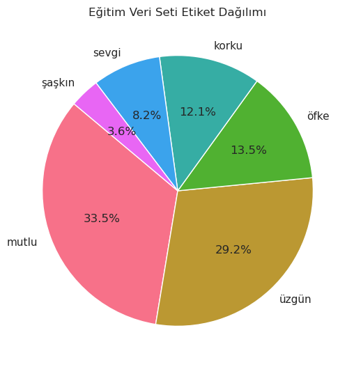
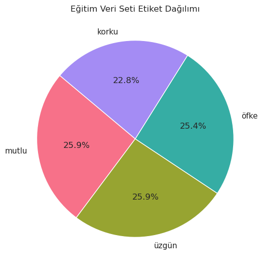
label_counts = train_df['label'].value_counts()
light_colors = sns.husl_palette(n_colors=len(label_counts)) # renk paleti olşuturulması
sns.set(style="whitegrid") # arka plan rengi
plt.figure(figsize=(6,6))
plt.pie(label_counts, labels=label_counts.index, autopct='%1.1f%%', startangle=140, colors=light_colors) # pasta grafiği oluşturulması
plt.title('Eğitim Veri Seti Etiket Dağılımı')
plt.show()
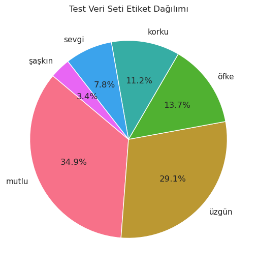
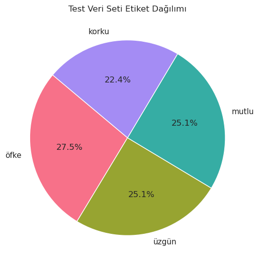
label_counts = test_df['label'].value_counts()
light_colors = sns.husl_palette(n_colors=len(label_counts)) # renk paleti olşuturulması
sns.set(style="whitegrid") # arka plan rengi
plt.figure(figsize=(6,6))
plt.pie(label_counts, labels=label_counts.index, autopct='%1.1f%%', startangle=140, colors=light_colors) # pasta grafiği oluşturulması
plt.title('Test Veri Seti Etiket Dağılımı')
plt.show()
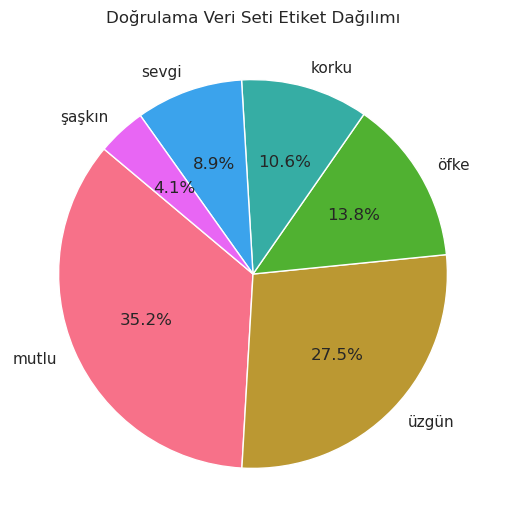
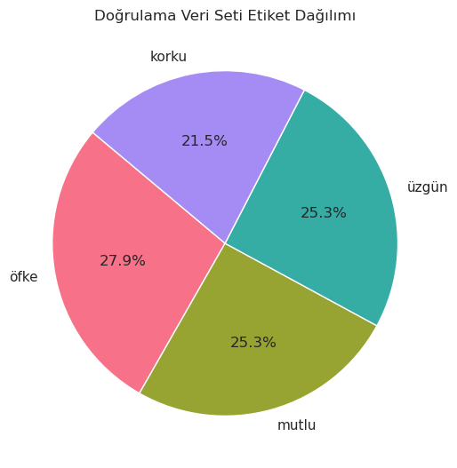
label_counts = val_df['label'].value_counts()
light_colors = sns.husl_palette(n_colors=len(label_counts)) # renk paleti olşuturulması
sns.set(style="whitegrid") # arka plan rengi
plt.figure(figsize=(6,6))
plt.pie(label_counts, labels=label_counts.index, autopct='%1.1f%%', startangle=140, colors=light_colors) # pasta grafiği oluşturulması
plt.title('Doğrulama Veri Seti Etiket Dağılımı')
plt.show()
Eğitim veri setindeki veriler dengesiz olduğu için ve veri setini daha dengeli hale getirmeliyim. Bunun için veri setindeki en az etiket sayısına sahip 2 etiket olan sevgi ve şaşkın etiketlerine sahip verileri çıkartacağım.
train_df = train_df[~train_df['label'].str.contains('sevgi')] # sevgi etiketine sahp verilerin çıkartılması
train_df = train_df[~train_df['label'].str.contains('şaşkın')] # şaşkın etiketine sahip verilerin çıkartlılması
Şimdi geriye kalan mutlu, üzgün, öfke ve korku etiketleri hala dengesiz bir şekilde dağılmış durumda. Bu etikerlerin dağılımını olabildiğince birbirine yaklaştırıyorum.
mutlu = train_df[train_df['label'] == 'mutlu'].sample(n=2200, random_state=20) # mutlu etiketine sahip rastgele 2200 veri
uzgun = train_df[train_df['label'] == 'üzgün'].sample(n=2200, random_state=20) # üzgün etiketine sahip rastgele 2200 veri
korku = train_df[train_df['label'] == 'korku'].sample(n=1937, random_state=20)
ofke = train_df[train_df['label'] == 'öfke'].sample(n=2160, random_state=20)

new_train_df = pd.concat([mutlu, uzgun, korku, ofke]) # rastgele seçilen bu verilerin birleştirilmesi

train_df = new_train_df.sample(frac=1, random_state=20).reset_index(drop=True) # birleştirilen verileri karıştırarak train_df yi yeniden oluşturuyorum
train_df.label.value_counts() # etiketlerin sayısı
label
mutlu    2200
üzgün    2200
öfke     2160
korku    1937
Name: count, dtype: int64
label_counts = train_df['label'].value_counts()
light_colors = sns.husl_palette(n_colors=len(label_counts))
sns.set(style="whitegrid")
plt.figure(figsize=(6, 6))
plt.pie(label_counts, labels=label_counts.index, autopct='%1.1f%%', startangle=140, colors=light_colors)
plt.title('Eğitim Veri Seti Etiket Dağılımı')
plt.show()
Artık eğitim veri seti daha dengeli hale geldi. Bu işlemlerin aynısını test_df ve val_df dataframeleri içinde yapacağım.
val_df.label.value_counts()
label
mutlu     704
üzgün     550
öfke      275
korku     212
sevgi     178
şaşkın     81
Name: count, dtype: int64
# sevgi ve şaşkın etiketlerinin çıkartılması
val_df = val_df[~val_df['label'].str.contains('sevgi')]
val_df = val_df[~val_df['label'].str.contains('şaşkın')]
mutlu = val_df[val_df['label'] == 'mutlu'].sample(n=250, random_state=20)
uzgun = val_df[val_df['label'] == 'üzgün'].sample(n=250, random_state=20)
korku = val_df[val_df['label'] == 'korku'].sample(n=212, random_state=20)
ofke = val_df[val_df['label'] == 'öfke'].sample(n=275, random_state=20)

df_sampled = pd.concat([mutlu, uzgun, korku, ofke])

val_df = df_sampled.sample(frac=1, random_state=20).reset_index(drop=True)
label_counts = val_df['label'].value_counts()
light_colors = sns.husl_palette(n_colors=len(label_counts))
sns.set(style="whitegrid")
plt.figure(figsize=(6, 6))
plt.pie(label_counts, labels=label_counts.index, autopct='%1.1f%%', startangle=140, colors=light_colors)
plt.title('Doğrulama Veri Seti Etiket Dağılımı')
plt.show()
test_df.label.value_counts()
label
mutlu     698
üzgün     582
öfke      274
korku     224
sevgi     155
şaşkın     67
Name: count, dtype: int64
# sevgi ve şaşkın etiketlerinin çıkartılması
test_df = test_df[~test_df['label'].str.contains('sevgi')]
test_df = test_df[~test_df['label'].str.contains('şaşkın')]
mutlu = test_df[test_df['label'] == 'mutlu'].sample(n=250, random_state=20)
uzgun = test_df[test_df['label'] == 'üzgün'].sample(n=250, random_state=20)
korku = test_df[test_df['label'] == 'korku'].sample(n=224, random_state=20)
ofke = test_df[test_df['label'] == 'öfke'].sample(n=274, random_state=20)

new_test_df = pd.concat([mutlu, uzgun, korku, ofke])

test_df = new_test_df.sample(frac=1, random_state=20).reset_index(drop=True)
label_counts = test_df['label'].value_counts()
light_colors = sns.husl_palette(n_colors=len(label_counts))
sns.set(style="whitegrid")
plt.figure(figsize=(6, 6))
plt.pie(label_counts, labels=label_counts.index, autopct='%1.1f%%', startangle=140, colors=light_colors)
plt.title('Test Veri Seti Etiket Dağılımı')
plt.show()
Split Data
train_text = train_df['sentence']
train_label = train_df['label']

val_text = val_df['sentence']
val_label = val_df['label']

test_text = test_df['sentence']
test_label = test_df['label']
Encoding
Şimdi bu etiketleri sayısal değerlere dönüştürüyorum.
encoder = LabelEncoder() # etiketlerin sayısal değerlere dönüştürülmesi
tr_label = encoder.fit_transform(train_label)
val_label = encoder.transform(val_label)
ts_label = encoder.transform(test_label)
Text Preprocessing
Şimdi de cümleleri Tokenizer modülü ile sayısal değerlere dönüştürerek model tarafından kullanılabilir hale getiriyorum.
tokenizer = Tokenizer(num_words=10000) # metinlerin sayısal değerlere dönüştürülmesi
tokenizer.fit_on_texts(train_text)

sequences = tokenizer.texts_to_sequences(train_text)
tr_x = pad_sequences(sequences, maxlen=50) # metinlerin boyutlarının eşitlenmesi
tr_y = to_categorical(tr_label, num_classes=4) # etiketlerin kategorik hale getirilmesi

sequences = tokenizer.texts_to_sequences(val_text)
val_x = pad_sequences(sequences, maxlen=50)
val_y = to_categorical(val_label, num_classes=4)

sequences = tokenizer.texts_to_sequences(test_text)
ts_x = pad_sequences(sequences, maxlen=50)
ts_y = to_categorical(ts_label, num_classes=4)
Building Deep Learning Model
max_words = 10000
max_len = 50
embedding_dim = 32
Model Architecture
# Branch 1
inputs1 = layers.Input(shape=(max_len,))  # inputs1 için giriş katmanı tanımlanması

branch1 = layers.Embedding(max_words, embedding_dim)(inputs1) # Embedding katmanı
branch1 = layers.Conv1D(64, 3, padding='same', activation='relu')(branch1) # Conv1D katmanı (64 filtre, 3 kernel boyutu)
branch1 = layers.BatchNormalization()(branch1) # BatchNormalization katmanı. Katman çıktılarını normalize eder.
branch1 = layers.ReLU()(branch1) # ReLU katmanı
branch1 = layers.Dropout(0.5)(branch1) # Dropout katmanı. Aşırı uyum (overfitting) önlemek için
branch1 = layers.GlobalMaxPooling1D()(branch1) # GlobalMaxPooling1D katmanı (en büyük değeri alır)

# Branch 2
inputs2 = layers.Input(shape=(max_len,))  # inputs2 için giriş katmanı tanımlanması

branch2 = layers.Embedding(max_words, embedding_dim)(inputs2)
branch2 = layers.Conv1D(64, 3, padding='same', activation='relu')(branch2)
branch2 = layers.BatchNormalization()(branch2)
branch2 = layers.ReLU()(branch2)
branch2 = layers.Dropout(0.5)(branch2)
branch2 = layers.GlobalMaxPooling1D()(branch2)

concatenated = layers.Concatenate()([branch1, branch2]) # Branch1 ve Branch2'nin birleştirilmesi

#Birleştirilen katmanların dense katmanı tarafından gizli katmana bağlanması
hid_layer = layers.Dense(128, activation='relu')(concatenated) # Gizli katman
dropout = layers.Dropout(0.3)(hid_layer) # Dropout katmanı. Overfitting önlemek için
output_layer = layers.Dense(4, activation='softmax')(dropout) # Çıkış katmanı

# Define the model with separate inputs
model = Model(inputs=[inputs1, inputs2], outputs=output_layer)
Compile Model
model.compile(optimizer='adamax', loss='categorical_crossentropy', metrics=['accuracy', Precision(), Recall()])

model.summary()
Model: "functional"
┏━━━━━━━━━━━━━━━━━━━━━┳━━━━━━━━━━━━━━━━━━━┳━━━━━━━━━━━━┳━━━━━━━━━━━━━━━━━━━┓
┃ Layer (type)        ┃ Output Shape      ┃    Param # ┃ Connected to      ┃
┡━━━━━━━━━━━━━━━━━━━━━╇━━━━━━━━━━━━━━━━━━━╇━━━━━━━━━━━━╇━━━━━━━━━━━━━━━━━━━┩
│ input_layer_2       │ (None, 50)        │          0 │ -                 │
│ (InputLayer)        │                   │            │                   │
├─────────────────────┼───────────────────┼────────────┼───────────────────┤
│ input_layer_3       │ (None, 50)        │          0 │ -                 │
│ (InputLayer)        │                   │            │                   │
├─────────────────────┼───────────────────┼────────────┼───────────────────┤
│ embedding_2         │ (None, 50, 32)    │    320,000 │ input_layer_2[0]… │
│ (Embedding)         │                   │            │                   │
├─────────────────────┼───────────────────┼────────────┼───────────────────┤
│ embedding_3         │ (None, 50, 32)    │    320,000 │ input_layer_3[0]… │
│ (Embedding)         │                   │            │                   │
├─────────────────────┼───────────────────┼────────────┼───────────────────┤
│ conv1d_2 (Conv1D)   │ (None, 50, 64)    │      6,208 │ embedding_2[0][0] │
├─────────────────────┼───────────────────┼────────────┼───────────────────┤
│ conv1d_3 (Conv1D)   │ (None, 50, 64)    │      6,208 │ embedding_3[0][0] │
├─────────────────────┼───────────────────┼────────────┼───────────────────┤
│ batch_normalizatio… │ (None, 50, 64)    │        256 │ conv1d_2[0][0]    │
│ (BatchNormalizatio… │                   │            │                   │
├─────────────────────┼───────────────────┼────────────┼───────────────────┤
│ batch_normalizatio… │ (None, 50, 64)    │        256 │ conv1d_3[0][0]    │
│ (BatchNormalizatio… │                   │            │                   │
├─────────────────────┼───────────────────┼────────────┼───────────────────┤
│ re_lu_2 (ReLU)      │ (None, 50, 64)    │          0 │ batch_normalizat… │
├─────────────────────┼───────────────────┼────────────┼───────────────────┤
│ re_lu_3 (ReLU)      │ (None, 50, 64)    │          0 │ batch_normalizat… │
├─────────────────────┼───────────────────┼────────────┼───────────────────┤
│ dropout_3 (Dropout) │ (None, 50, 64)    │          0 │ re_lu_2[0][0]     │
├─────────────────────┼───────────────────┼────────────┼───────────────────┤
│ dropout_4 (Dropout) │ (None, 50, 64)    │          0 │ re_lu_3[0][0]     │
├─────────────────────┼───────────────────┼────────────┼───────────────────┤
│ global_max_pooling… │ (None, 64)        │          0 │ dropout_3[0][0]   │
│ (GlobalMaxPooling1… │                   │            │                   │
├─────────────────────┼───────────────────┼────────────┼───────────────────┤
│ global_max_pooling… │ (None, 64)        │          0 │ dropout_4[0][0]   │
│ (GlobalMaxPooling1… │                   │            │                   │
├─────────────────────┼───────────────────┼────────────┼───────────────────┤
│ concatenate_1       │ (None, 128)       │          0 │ global_max_pooli… │
│ (Concatenate)       │                   │            │ global_max_pooli… │
├─────────────────────┼───────────────────┼────────────┼───────────────────┤
│ dense_2 (Dense)     │ (None, 128)       │     16,512 │ concatenate_1[0]… │
├─────────────────────┼───────────────────┼────────────┼───────────────────┤
│ dropout_5 (Dropout) │ (None, 128)       │          0 │ dense_2[0][0]     │
├─────────────────────┼───────────────────┼────────────┼───────────────────┤
│ dense_3 (Dense)     │ (None, 4)         │        516 │ dropout_5[0][0]   │
└─────────────────────┴───────────────────┴────────────┴───────────────────┘
Training The Model
batch_size = 50
epochs = 10
history = model.fit([tr_x, tr_x], tr_y, epochs=epochs, batch_size=batch_size, validation_data=([val_x, val_x], val_y))
Epoch 1/10
170/170 ━━━━━━━━━━━━━━━━━━━━ 14s 38ms/step - accuracy: 0.2675 - loss: 1.5784 - precision_1: 0.2685 - recall_1: 0.0702 - val_accuracy: 0.2644 - val_loss: 1.3848 - val_precision_1: 0.0000e+00 - val_recall_1: 0.0000e+00
Epoch 2/10
170/170 ━━━━━━━━━━━━━━━━━━━━ 2s 9ms/step - accuracy: 0.3341 - loss: 1.3538 - precision_1: 0.5342 - recall_1: 0.0124 - val_accuracy: 0.3556 - val_loss: 1.3767 - val_precision_1: 0.0000e+00 - val_recall_1: 0.0000e+00
Epoch 3/10
170/170 ━━━━━━━━━━━━━━━━━━━━ 1s 5ms/step - accuracy: 0.3941 - loss: 1.2952 - precision_1: 0.6062 - recall_1: 0.0445 - val_accuracy: 0.4590 - val_loss: 1.3262 - val_precision_1: 0.0000e+00 - val_recall_1: 0.0000e+00
Epoch 4/10
170/170 ━━━━━━━━━━━━━━━━━━━━ 1s 6ms/step - accuracy: 0.5009 - loss: 1.1432 - precision_1: 0.7271 - recall_1: 0.2051 - val_accuracy: 0.5370 - val_loss: 1.1861 - val_precision_1: 0.9302 - val_recall_1: 0.0811
Epoch 5/10
170/170 ━━━━━━━━━━━━━━━━━━━━ 1s 5ms/step - accuracy: 0.5728 - loss: 1.0054 - precision_1: 0.7464 - recall_1: 0.3528 - val_accuracy: 0.5998 - val_loss: 1.0297 - val_precision_1: 0.8799 - val_recall_1: 0.2523
Epoch 6/10
170/170 ━━━━━━━━━━━━━━━━━━━━ 1s 6ms/step - accuracy: 0.6539 - loss: 0.8436 - precision_1: 0.7765 - recall_1: 0.5050 - val_accuracy: 0.6353 - val_loss: 0.9254 - val_precision_1: 0.8305 - val_recall_1: 0.3972
Epoch 7/10
170/170 ━━━━━━━━━━━━━━━━━━━━ 1s 7ms/step - accuracy: 0.7281 - loss: 0.7166 - precision_1: 0.8066 - recall_1: 0.6189 - val_accuracy: 0.6657 - val_loss: 0.8461 - val_precision_1: 0.8419 - val_recall_1: 0.4965
Epoch 8/10
170/170 ━━━━━━━━━━━━━━━━━━━━ 1s 6ms/step - accuracy: 0.7787 - loss: 0.5958 - precision_1: 0.8340 - recall_1: 0.6916 - val_accuracy: 0.6991 - val_loss: 0.7823 - val_precision_1: 0.8294 - val_recall_1: 0.5714
Epoch 9/10
170/170 ━━━━━━━━━━━━━━━━━━━━ 1s 7ms/step - accuracy: 0.8125 - loss: 0.5114 - precision_1: 0.8518 - recall_1: 0.7635 - val_accuracy: 0.7143 - val_loss: 0.7323 - val_precision_1: 0.8171 - val_recall_1: 0.6109
Epoch 10/10
170/170 ━━━━━━━━━━━━━━━━━━━━ 1s 5ms/step - accuracy: 0.8342 - loss: 0.4520 - precision_1: 0.8707 - recall_1: 0.7920 - val_accuracy: 0.7285 - val_loss: 0.7097 - val_precision_1: 0.8307 - val_recall_1: 0.6363
Evaluation and Visullize Results
(loss, accuracy, percision, recall) = model.evaluate([tr_x, tr_x], tr_y)
print(f'Loss: {round(loss, 2)}, Accuracy: {round(accuracy, 2)}, Precision: {round(percision, 2)}, Recall: {round(recall, 2)}')
266/266 ━━━━━━━━━━━━━━━━━━━━ 1s 4ms/step - accuracy: 0.9416 - loss: 0.2891 - precision_1: 0.9652 - recall_1: 0.8972
Loss: 0.3, Accuracy: 0.93, Precision: 0.96, Recall: 0.89
(loss, accuracy, percision, recall) = model.evaluate([ts_x, ts_x], ts_y)
print(f'Loss: {round(loss, 2)}, Accuracy: {round(accuracy, 2)}, Precision: {round(percision, 2)}, Recall: {round(recall, 2)}')
16/32 ━━━━━━━━━━━━━━━━━━━━ 0s 3ms/step - accuracy: 0.6958 - loss: 0.7529 - precision_1: 0.7563 - recall_1: 0.5804
32/32 ━━━━━━━━━━━━━━━━━━━━ 0s 11ms/step - accuracy: 0.7036 - loss: 0.7366 - precision_1: 0.7747 - recall_1: 0.5994
Loss: 0.74, Accuracy: 0.7, Precision: 0.79, Recall: 0.62
history.history.keys()
dict_keys(['accuracy', 'loss', 'precision_1', 'recall_1', 'val_accuracy', 'val_loss', 'val_precision_1', 'val_recall_1'])
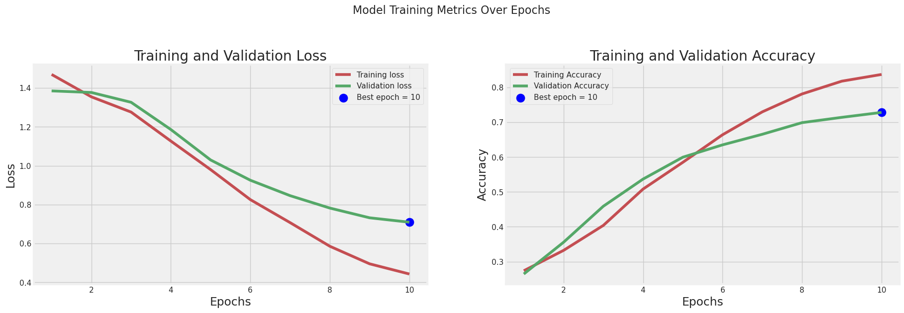
Visullize Results
tr_acc = history.history['accuracy']
tr_loss = history.history['loss']
val_acc = history.history['val_accuracy']
val_loss = history.history['val_loss']

index_loss = np.argmin(val_loss)
val_lowest = val_loss[index_loss]
index_acc = np.argmax(val_acc)
acc_highest = val_acc[index_acc]


Epochs = [i + 1 for i in range(len(tr_acc))]
loss_label = f'Best epoch = {str(index_loss + 1)}'
acc_label = f'Best epoch = {str(index_acc + 1)}'


plt.figure(figsize=(20, 12))
plt.style.use('fivethirtyeight')


plt.subplot(2, 2, 1)
plt.plot(Epochs, tr_loss, 'r', label='Training loss')
plt.plot(Epochs, val_loss, 'g', label='Validation loss')
plt.scatter(index_loss + 1, val_lowest, s=150, c='blue', label=loss_label)
plt.title('Training and Validation Loss')
plt.xlabel('Epochs')
plt.ylabel('Loss')
plt.legend()
plt.grid(True)

plt.subplot(2, 2, 2)
plt.plot(Epochs, tr_acc, 'r', label='Training Accuracy')
plt.plot(Epochs, val_acc, 'g', label='Validation Accuracy')
plt.scatter(index_acc + 1, acc_highest, s=150, c='blue', label=acc_label)
plt.title('Training and Validation Accuracy')
plt.xlabel('Epochs')
plt.ylabel('Accuracy')
plt.legend()
plt.grid(True)


plt.suptitle('Model Training Metrics Over Epochs', fontsize=16)
plt.show()
y_true=[] # gerçek etiketlerin tutulacağı liste
for i in range(len(ts_y)): # gerçek etiketlerin alınması
    x = np.argmax(ts_y[i])
    y_true.append(x)


preds = model.predict([ts_x, ts_x]) # tahminlerin alınması
y_pred = np.argmax(preds, axis=1) # tahminlerin en yüksek değerli indexlerinin alınması
y_true = np.argmax(ts_y, axis=1) # gerçek etiketlerin en yüksek değerli indexlerinin alınması
y_pred
32/32 ━━━━━━━━━━━━━━━━━━━━ 1s 10ms/step
array([2, 0, 3, 3, 1, 2, 0, 0, 2, 1, 2, 3, 3, 1, 3, 3, 3, 3, 2, 3, 3, 1,
       1, 3, 0, 1, 2, 1, 3, 0, 3, 0, 3, 2, 3, 1, 3, 3, 2, 0, 0, 2, 2, 3,
       0, 0, 1, 2, 3, 0, 3, 1, 1, 1, 0, 3, 1, 1, 3, 1, 3, 3, 0, 2, 1, 3,
       2, 3, 1, 0, 2, 1, 3, 2, 2, 0, 0, 2, 1, 1, 3, 0, 3, 3, 0, 1, 2, 1,
       1, 3, 1, 1, 3, 0, 3, 0, 3, 3, 2, 1, 3, 0, 2, 0, 2, 3, 2, 1, 3, 2,
       3, 2, 3, 1, 3, 2, 3, 0, 1, 1, 3, 3, 3, 0, 3, 0, 3, 2, 1, 1, 3, 2,
       2, 3, 1, 3, 3, 2, 1, 2, 1, 3, 0, 1, 2, 2, 2, 1, 0, 0, 1, 2, 1, 1,
       2, 2, 3, 0, 2, 3, 1, 3, 0, 0, 2, 3, 2, 1, 2, 2, 1, 2, 0, 3, 1, 0,
       1, 0, 3, 1, 3, 1, 3, 0, 3, 1, 1, 1, 0, 1, 2, 2, 1, 3, 3, 3, 1, 2,
       2, 1, 0, 2, 0, 1, 1, 2, 3, 3, 2, 3, 3, 0, 0, 2, 2, 3, 3, 3, 1, 3,
       1, 3, 3, 0, 0, 2, 0, 1, 2, 2, 2, 2, 0, 0, 3, 3, 2, 0, 1, 3, 1, 0,
       0, 1, 1, 3, 1, 2, 2, 2, 0, 3, 1, 0, 3, 2, 3, 3, 0, 3, 1, 2, 1, 2,
       3, 2, 1, 2, 2, 0, 1, 1, 3, 3, 3, 3, 1, 3, 0, 3, 2, 0, 3, 0, 1, 0,
       3, 3, 0, 0, 3, 2, 1, 0, 3, 3, 2, 1, 3, 3, 1, 3, 2, 1, 2, 1, 2, 3,
       3, 3, 2, 3, 3, 3, 0, 0, 3, 0, 2, 1, 2, 3, 1, 3, 0, 3, 1, 3, 1, 2,
       1, 3, 3, 0, 3, 0, 3, 1, 3, 0, 1, 1, 3, 3, 3, 3, 0, 1, 3, 2, 2, 2,
       1, 1, 2, 3, 0, 2, 2, 1, 3, 3, 3, 3, 0, 3, 0, 0, 1, 2, 3, 3, 1, 2,
       2, 0, 1, 2, 2, 2, 1, 3, 1, 1, 2, 3, 2, 0, 2, 1, 3, 0, 2, 3, 0, 3,
       0, 0, 2, 0, 3, 3, 2, 3, 2, 3, 3, 2, 1, 0, 2, 3, 1, 3, 2, 3, 1, 0,
       0, 2, 2, 0, 3, 0, 3, 3, 0, 3, 3, 2, 0, 2, 2, 1, 3, 3, 0, 1, 3, 0,
       2, 2, 2, 1, 2, 3, 1, 2, 1, 0, 3, 2, 1, 0, 3, 1, 0, 2, 3, 2, 0, 1,
       1, 2, 0, 0, 1, 1, 3, 1, 2, 0, 3, 0, 3, 3, 3, 1, 3, 1, 1, 2, 1, 3,
       0, 3, 0, 0, 2, 2, 0, 0, 3, 0, 2, 0, 2, 1, 2, 0, 1, 1, 3, 1, 3, 2,
       1, 0, 2, 1, 3, 3, 3, 1, 2, 1, 1, 3, 2, 1, 3, 1, 1, 2, 2, 3, 3, 3,
       1, 0, 2, 3, 1, 0, 3, 3, 0, 2, 3, 0, 0, 2, 3, 0, 3, 0, 2, 0, 3, 1,
...
       3, 2, 1, 2, 1, 3, 1, 1, 3, 3, 0, 3, 2, 0, 3, 3, 2, 0, 3, 2, 0, 0,
       0, 2, 0, 2, 1, 2, 3, 2, 2, 2, 3, 0, 0, 3, 3, 2, 3, 0, 1, 0, 2, 2,
       2, 3, 0, 3, 3, 2, 0, 2, 2, 2, 1, 3, 2, 2, 3, 3, 3, 2, 3, 3, 3, 1,
       2, 1, 3, 2, 0, 1, 1, 2, 2, 2, 3, 3, 3, 0, 2, 3, 3, 3, 1, 2, 2, 2,
       3, 3, 1, 2, 3, 2, 3, 3])
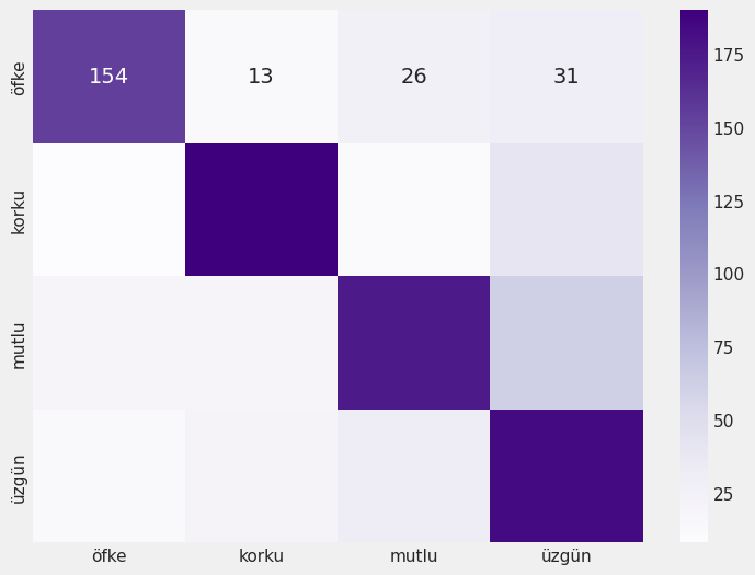
plt.figure(figsize=(8,6))
emotions = {0: 'öfke', 1: 'korku', 2: 'mutlu', 3:'üzgün'}
emotions = list(emotions.values())
cm = confusion_matrix(y_true, y_pred.ravel())
sns.heatmap(cm, annot=True, fmt='d', cmap='Purples', xticklabels=emotions, yticklabels=emotions)
Classification Report
clr = classification_report(y_true, y_pred)
print(clr)
              precision    recall  f1-score   support

           0       0.79      0.69      0.74       224
           1       0.78      0.76      0.77       250
           2       0.72      0.64      0.67       274
           3       0.58      0.74      0.65       250

    accuracy                           0.70       998
   macro avg       0.72      0.70      0.71       998
weighted avg       0.72      0.70      0.71       998
Save Model
Eğitilmiş olan tokenizatörün ve modelin kaydedilmesi
with open('tokenizer.pkl', 'wb') as tokenizer_file: # tokenizer nesnesinin kaydedilmesi
    pickle.dump(tokenizer, tokenizer_file)

model.save('emotions_detect_model.h5')
Prediction Function
# modülleri tekrardan import etmemin sebebi, modeli tekrar eğitmeden kaydedilen modeli kullanmak için

from tensorflow.keras.preprocessing.sequence import pad_sequences
from tensorflow.keras.models import load_model
import pickle
import matplotlib.pyplot as plt
import numpy as np
def predict(text, model_path, token_path):
model = load_model(model_path)
with open(token_path, 'rb') as f:
tokenizer = pickle.load(f)
sequences = tokenizer.texts_to_sequences([text]) # Tahmin edilecek metni önceden eğitilen tokenizer ile sayısal değerlere dönüştürülmesi
x_new = pad_sequences(sequences, maxlen=50) # Metinlerin boyutlarının eşitlenmesi
predictions = model.predict([x_new, x_new]) # Tahmin işlemi
emotions = {0: 'üzgün', 1: 'mutlu', 2: 'korku', 3:'öfke'}
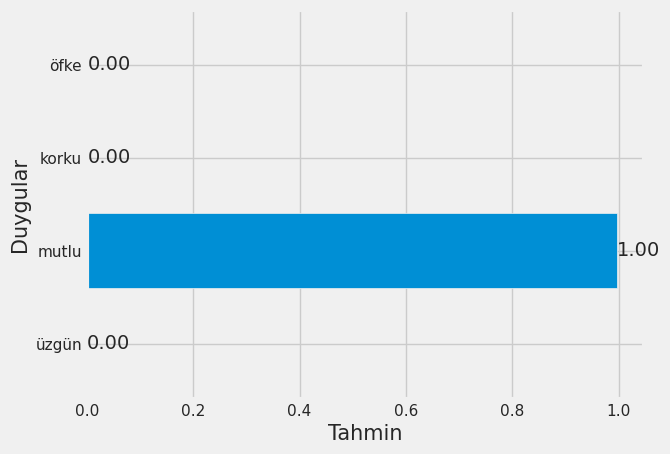
# Tahmin sonuçlarının görselleştirilmesi
label = list(emotions.values())
probs = list(predictions[0])
labels = label
plt.subplot(1, 1, 1)
bars = plt.barh(labels, probs)
plt.xlabel('Tahmin', fontsize=15)
plt.ylabel('Duygular', fontsize=15)
ax = plt.gca()
ax.bar_label(bars, fmt = '%.2f')
plt.show()
return emotions[np.argmax(predictions)] # En yüksek değerli indexin alınması ve duygunun döndürülmesi
Prediction
txt = 'Projeyi bitirdiğim için kendimi harika hissediyorum'
predict(txt, 'emotions_detect_model.h5', 'tokenizer.pkl')
1/1 ━━━━━━━━━━━━━━━━━━━━ 0s 330ms/step
'mutlu'