Multiple Linear Regression Example
Categorized under Machine Learning tagged Prediction Last modified at:

Multiple Linear Regression Example
- Dataset
- Import Libraries
- Read and Preprocessing Data
- Train Model
- Predict
- Visualize results of the model
- Backward Elimination
- Re-build Model
- Re-predict
- Visualize the results
- Results
Bu yazıda, hava durumu, sıcaklık, rüzgar durumu gibi değişkenler kullanarak nem (humidity) seviyesini tahmin etmeyi amaçladığımız bir çoklu doğrusal regresyon çalışmasını ele alacağız.
Dataset
Import Libraries
import numpy as np
import pandas as pd
import matplotlib.pyplot as plt
import seaborn as sbn
Read and Preprocessing Data
Read Data
data = pd.read_csv('tennis.csv')

print(data.head(15))
      outlook  temperature  humidity  windy play
0      sunny           85        85  False   no
1      sunny           80        90   True   no
2   overcast           83        86  False  yes
3      rainy           70        96  False  yes
4      rainy           68        80  False  yes
5      rainy           65        70   True   no
6   overcast           64        65   True  yes
7      sunny           72        95  False   no
8      sunny           69        70  False  yes
9      rainy           75        80  False  yes
10     sunny           75        70   True  yes
11  overcast           72        90   True  yes
12  overcast           81        75  False  yes
13     rainy           71        91   True   no
Analysis of Data
sbn.pairplot(data) # for better visualization
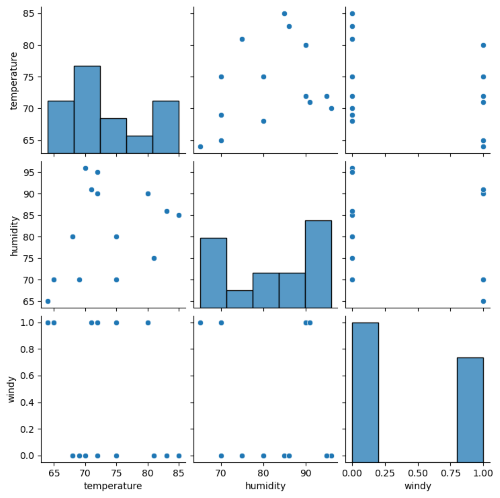
print(data.describe())
       temperature   humidity
count    14.000000  14.000000
mean     73.571429  81.642857
std       6.571667  10.285218
min      64.000000  65.000000
25%      69.250000  71.250000
50%      72.000000  82.500000
75%      78.750000  90.000000
max      85.000000  96.000000
Split Data
outlook = data.iloc[:, 0:1].values
temperature = data.iloc[:, 1:2].values
humidity = data.iloc[:, 2:3].values
wind = data.iloc[:, 3:4].values
play = data.iloc[:, 4:5].values
Encoding
from sklearn.preprocessing import LabelEncoder, OneHotEncoder

le = LabelEncoder()
ohe = OneHotEncoder()

outlook = ohe.fit_transform(outlook).toarray()
wind = le.fit_transform(wind).reshape(-1, 1)
play = le.fit_transform(play).reshape(-1, 1)
Concatenate data
last_data = np.concatenate([outlook, temperature, humidity, wind, play], axis=1)
# Convert to DataFrame from numpy array
last_data = pd.DataFrame(data= last_data, columns=['overcast', 'rainy', 'sunny', 'temperature', 'humidity', 'windy', 'play'])

print(last_data.head(15))
    overcast  rainy  sunny  temperature  humidity  windy  play
0        0.0    0.0    1.0         85.0      85.0    0.0   0.0
1        0.0    0.0    1.0         80.0      90.0    1.0   0.0
2        1.0    0.0    0.0         83.0      86.0    0.0   1.0
3        0.0    1.0    0.0         70.0      96.0    0.0   1.0
4        0.0    1.0    0.0         68.0      80.0    0.0   1.0
5        0.0    1.0    0.0         65.0      70.0    1.0   0.0
6        1.0    0.0    0.0         64.0      65.0    1.0   1.0
7        0.0    0.0    1.0         72.0      95.0    0.0   0.0
8        0.0    0.0    1.0         69.0      70.0    0.0   1.0
9        0.0    1.0    0.0         75.0      80.0    0.0   1.0
10       0.0    0.0    1.0         75.0      70.0    1.0   1.0
11       1.0    0.0    0.0         72.0      90.0    1.0   1.0
12       1.0    0.0    0.0         81.0      75.0    0.0   1.0
13       0.0    1.0    0.0         71.0      91.0    1.0   0.0
Train Test Split
xbağımsız değişkeni; overcast, rainy, sunny, temperature, windy, playybağımlı değişkeni; humidty
olacak şekilde verisetini ayırıyorum.
from sklearn.model_selection import train_test_split

x = last_data.iloc[:, 0:7].values
x = pd.DataFrame(x)
x = x.drop(4, axis=1)

y = last_data.iloc[:, 4].values

x_train, x_test, y_train, y_test = train_test_split(x, y, test_size=0.33, random_state=0)
Train Model
from sklearn.linear_model import LinearRegression

lr = LinearRegression()
lr.fit(x_train, y_train)
Predict
y_pred = lr.predict(x_test)

for i in range(len(y_pred)):
    print('Predicted: ', y_pred[i], '\tReal: ', y_test[i])
Predicted:  84.45365572826714 	Real:  70.0
Predicted:  63.938399539435814 	Real:  65.0
Predicted:  85.76050662061026 	Real:  80.0
Predicted:  64.21013241220496 	Real:  90.0
Predicted:  75.06793321819228 	Real:  86.0
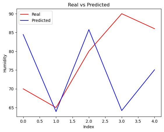
Visualize results of the model
plt.plot(y_test, color='red', label='Real')
plt.plot(y_pred, color='blue', label='Predicted')
plt.title('Real vs Predicted')
plt.xlabel('Index')
plt.ylabel('Humidity')
plt.legend()
plt.show()
Backward Elimination
Adding constant
constant = np.ones((len(x), 1)).astype(int)
x = np.append(arr=constant, values=x, axis=1)
Backward Elimination
import statsmodels.api as sm

x_opt = x[:, [0, 1, 2, 3, 4, 5, 6]]
model = sm.OLS(endog=y, exog=x_opt).fit()

print(model.summary())
                            OLS Regression Results
==============================================================================
Dep. Variable:                      y   R-squared:                       0.294
Model:                            OLS   Adj. R-squared:                 -0.148
Method:                 Least Squares   F-statistic:                    0.6653
Date:                Tue, 06 Aug 2024   Prob (F-statistic):              0.661
Time:                        19:03:32   Log-Likelihood:                -49.542
No. Observations:                  14   AIC:                             111.1
Df Residuals:                       8   BIC:                             114.9
Df Model:                           5
Covariance Type:            nonrobust
==============================================================================
                 coef    std err          t      P>|t|      [0.025      0.975]
------------------------------------------------------------------------------
const         39.3630     35.781      1.100      0.303     -43.149     121.875
x1            13.0261     15.032      0.867      0.411     -21.637      47.689
x2            16.2707     10.134      1.605      0.147      -7.099      39.641
x3            10.0661     13.179      0.764      0.467     -20.325      40.457
x4             0.4920      0.597      0.825      0.433      -0.884       1.868
x5            -4.0286      7.229     -0.557      0.593     -20.698      12.641
x6            -8.2778      8.029     -1.031      0.333     -26.793      10.237
==============================================================================
Omnibus:                        0.935   Durbin-Watson:                   2.416
Prob(Omnibus):                  0.627   Jarque-Bera (JB):                0.823
Skew:                           0.389   Prob(JB):                        0.663
Eliminate x5
x_opt = x_opt[:, [0, 1, 2, 3, 4, 6]]
model = sm.OLS(endog=y, exog=x_opt).fit()

print(model.summary())
                            OLS Regression Results
==============================================================================
Dep. Variable:                      y   R-squared:                       0.266
Model:                            OLS   Adj. R-squared:                 -0.060
Method:                 Least Squares   F-statistic:                    0.8165
Date:                Wed, 07 Aug 2024   Prob (F-statistic):              0.546
Time:                        00:04:08   Log-Likelihood:                -49.809
No. Observations:                  14   AIC:                             109.6
Df Residuals:                       9   BIC:                             112.8
Df Model:                           4
Covariance Type:            nonrobust
==============================================================================
                 coef    std err          t      P>|t|      [0.025      0.975]
------------------------------------------------------------------------------
const         28.4191     28.743      0.989      0.349     -36.601      93.440
x1             8.2373     11.852      0.695      0.505     -18.573      35.047
x2            13.4944      8.481      1.591      0.146      -5.690      32.679
x3             6.6873     11.245      0.595      0.567     -18.750      32.125
x4             0.6484      0.506      1.282      0.232      -0.496       1.793
x5            -6.2865      6.909     -0.910      0.387     -21.916       9.343
==============================================================================
Omnibus:                        0.887   Durbin-Watson:                   2.360
Prob(Omnibus):                  0.642   Jarque-Bera (JB):                0.810
Skew:                           0.424   Prob(JB):                        0.667
Kurtosis:                       2.181   Cond. No.                     8.20e+17
Re-build Model
x = x_opt

x_train, x_test, y_train, y_test = train_test_split(x, y, test_size=0.33, random_state=0)

lr = LinearRegression()
lr.fit(x_train, y_train)
Re-predict
y_pred = lr.predict(x_test)

for i in range(len(y_pred)):
    print('Predicted: ', y_pred[i], '\tReal: ', y_test[i])
Predicted:  77.98135141680795 	Real:  70.0
Predicted:  68.29304916444661 	Real:  65.0
Predicted:  81.05037539355777 	Real:  80.0
Predicted:  71.44926132235409 	Real:  90.0
Predicted:  75.78905303947685 	Real:  86.0
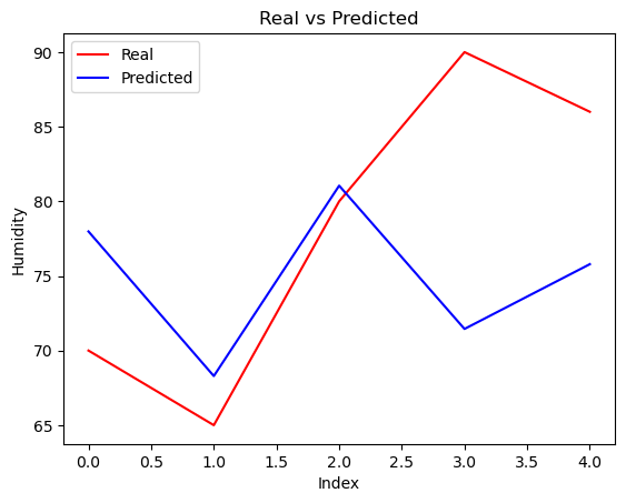
Visualize the results
plt.plot(y_test, color='red', label='Real')
plt.plot(y_pred, color='blue', label='Predicted')
plt.title('Real vs Predicted')
plt.xlabel('Index')
plt.ylabel('Humidity')
plt.legend()
plt.show()
Results
Bu çalışmada, hava durumu ve diğer çevresel değişkenleri kullanarak nem seviyesini tahmin eden bir çoklu doğrusal regresyon modeli geliştirdik ve değerlendirdik. Çoklu doğrusal regresyon modeli, nem tahmininde makul bir doğruluk sağlamıştır. Ayrıca, spor aktiviteleri gibi hava koşullarının kritik rol oynadığı alanlarda veri bilimi ve makine öğrenmesi uygulamalarının nasıl değer katabileceğini de ortaya koymaktadır.